Local Gaussian Filter and Adaptive Morphology Operation

Local Gaussian Filter and Adaptive Morphology Operation

Authors: P. Markowicz, P. Spurek

History: 2013/11/26: First version

Bugs: 0 bug(s) listed.

Plugin: LocalGaussianFilter_AdaptiveMorphologyOperation-1.0.0.jar

Installation: Download LocalGaussianFilter_AdaptiveMorphologyOperation-1.0.0.jar to the plugins folder (restart ImageJ) and there will be new commands:

Plugins/Adaptive Morphology,

Plugins/Gaussina filter.

References: P. Spurek, A. Chaikouskaya, J. Tabor, E. Zając A local Gaussian ﬁlter and adaptive morphology as tools for completing partially discontinuous curves, CISIM 2014, LNCS 8838, pp. 559–570, 2014 (Please cite as "Bibtex")
Description:

Local Gaussian Filter

Gaussian blur (also known as Gaussian smoothing) is the result of blurring of an image by the Gaussian function. For processing images, one needs a two-dimensional Gaussian density distribution. The normal random variable with the mean equal to zero and the covariance matrix $\Sigma$ has a density

$\frac{1}{2\pi%20\sqrt{%20\det(\Sigma)}}\exp\left(-\frac{1}{2}|%20x%20|_{\Sigma}^{2}\right)$
where by
${{| x |}_{\Sigma}}^{2} : = x^T\Sigma^{-1}x$
we denote the Mahalanobis norm of $x \in \mathbb{R}^2$ .
An image with dimensions $m \times n$ is interpreted as a function $J : [0,m-1] \times [0,n-1] \to [0,1]$ , where $J(k_1,k_2 )$ describes the intensity of the pixel with coordinates $(k_1,k_2 )$ .
Local Gaussian blur is obtained by replacing each pixel with coordinates $(k_1,k_2 )$ using the formula

$\left( g_{\Sigma} * J \right) (k_1,k_2)$ ,
where $\Sigma$ is the local covariance matrix for a circular neighborhood.
We need one parameter: radius r of circular neighborhood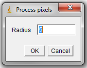

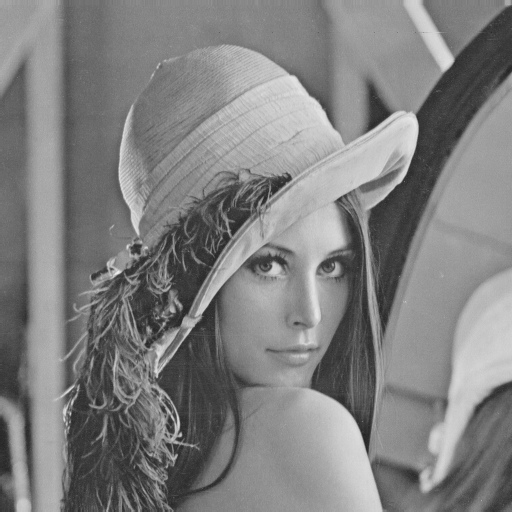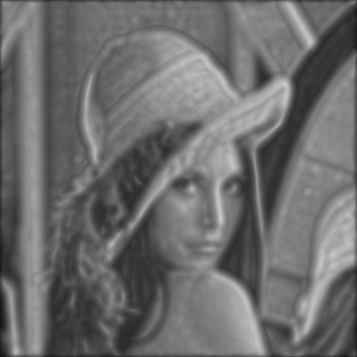
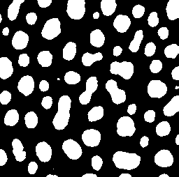
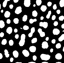
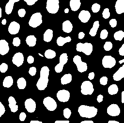
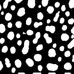
Example: The effect of Local Gaussian Filter on Classical Lena Picture with $r=10$

Adaptive morphology operation

Similarly as in the local Gaussian filter, adaptive morphology operation uses local properties of images. More precisely, a covariance matrix is employed to fit the size and orientation of elliptical structural elements.

We implement dilatation (black color describe background and white describe elements of foreground).

Let us consider the set presented below. Let $r=2$ be arbitrarily fixed. The behavior of an adaptive morphology is described for two points, which are marked black.
We use coordinates of points from the neighborhood to determine a covariance matrix. In this example, elements of the curve are marked in light gray. As we see structural element is different in each of points.
The most important property is that this operation do not expand the set in all directions. To emphasize this effect we added the parameter $\alpha$ . The morphology operation is applied if proportion between parameters $a,b$ of estimated elipses is lower then $\alpha$ .
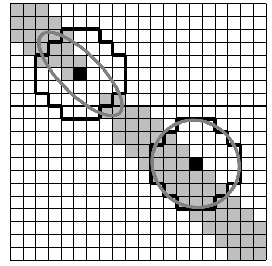
We need two parameters:

radius r of circular neighborhood

proportion between parameters $a,b:\alpha$

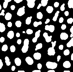
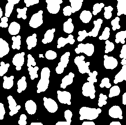
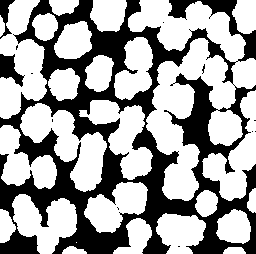
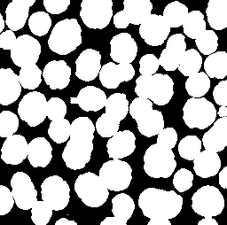
Example: The effect of Adaptive morphology on Blobs image with $r=10$ and different parameter $\alpha$

Blobs image thresholding by Otsu algorithm. $r=5$ and $\alpha=0.4$ $r=5$ and $\alpha=0.5$ $r=5$ and $\alpha=0.6$

$r=5$ and $\alpha=0.7$ $r=5$ and $\alpha=0.8$ $r=5$ and $\alpha=0.9$ $r=5$ and $\alpha=1$

|Plugins | Home |